
Scientific plots that are pieces of art.
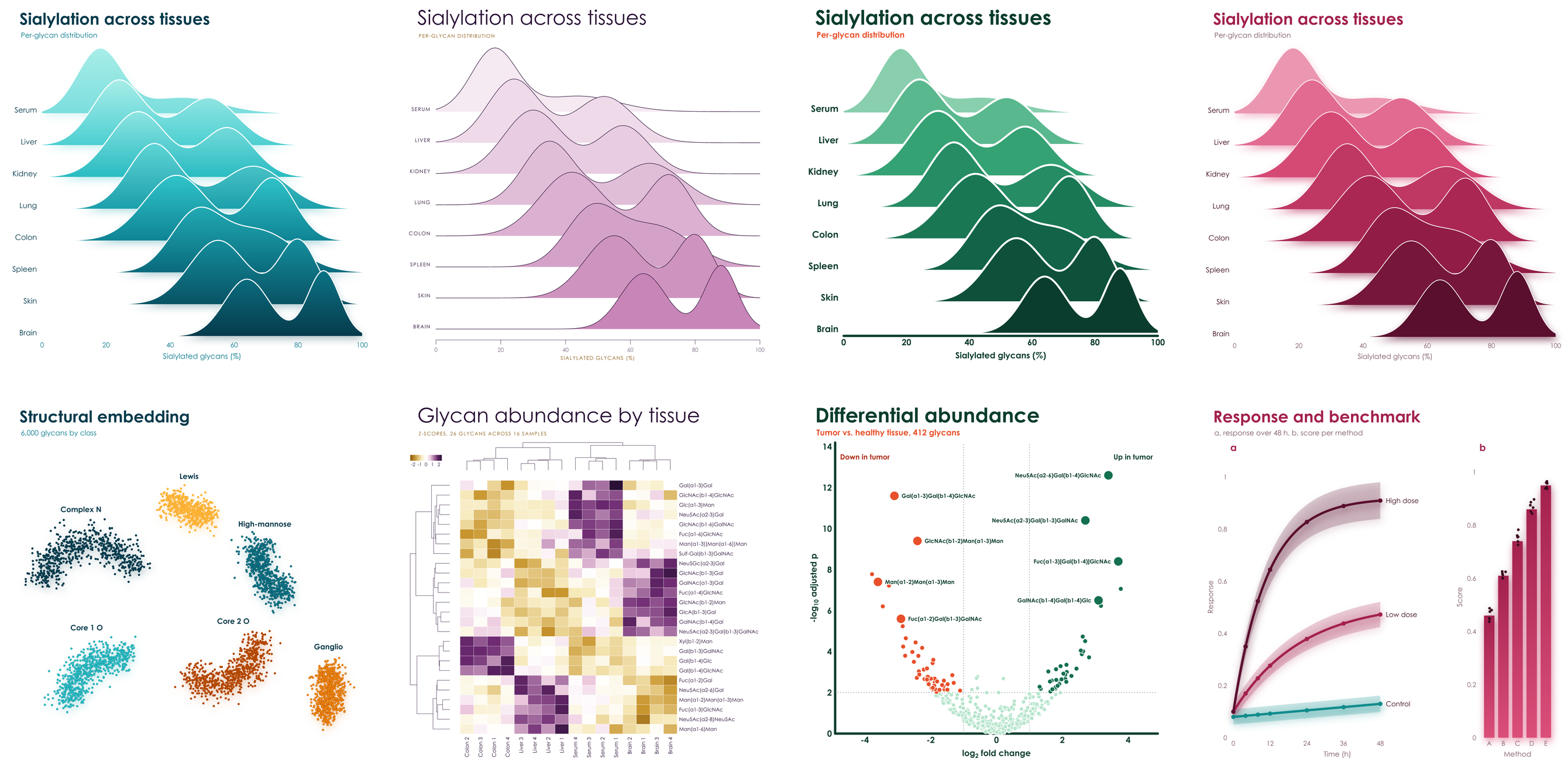
Pick a palette. It brings its own colors, type, axes, and special effects.
pip install viscose              # numpy and glycorender are all it needs
pip install "viscose[cluster]" # adds scipy for clustermapsimport viscose as vc
fig, ax = vc.subplots(palette = 'aura')
fig.suptitle('Differential abundance', 'Tumor vs. healthy tissue, 412 glycans')
ax.scatter(x, y, hue = direction)
ax.axhline(2)
ax.set_xlabel('log_{2} fold change')
ax.set_ylabel('-log_{10} adjusted p')
fig.save('volcano.pdf')Same data, same code, and only palette changes. Spheres become rings, gradients become solid shapes, hairline axes become
heavy rounded ones, and titles go from light and wide to bold and tight. No styling code, no rcParams, and no theme files.
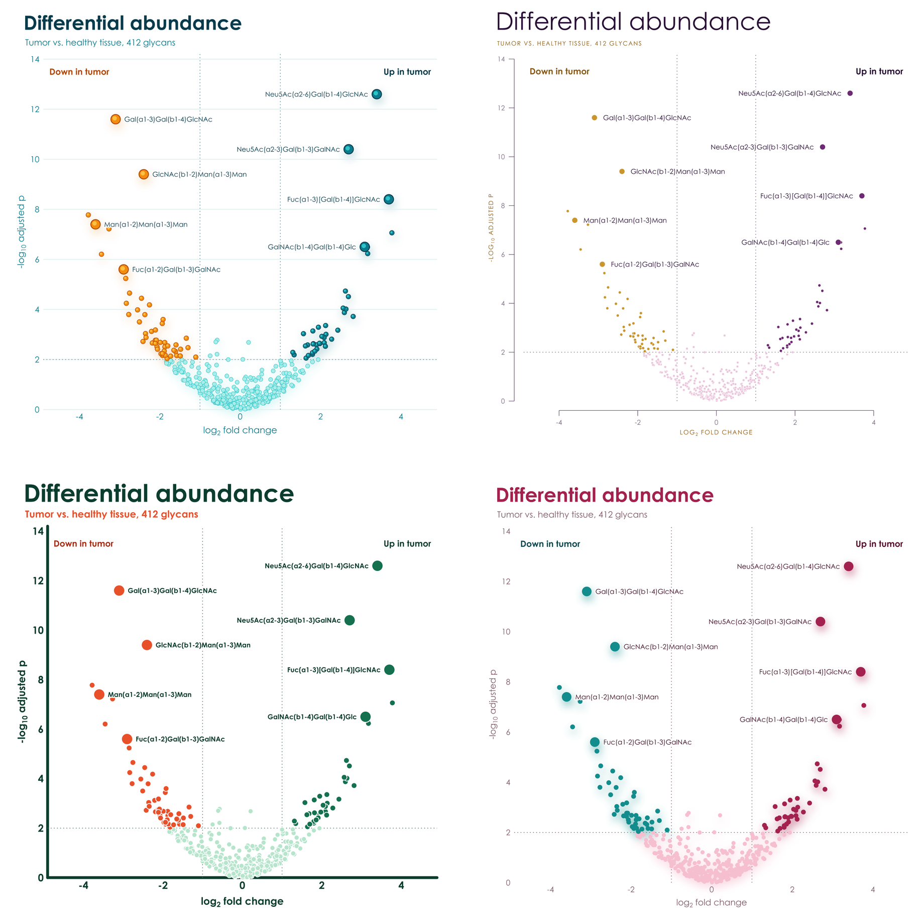
Each palette has two hues in four shades, and effects to match. Few colors, in shades of those few colors, on white: figures that look composed in a paper and striking on a slide.
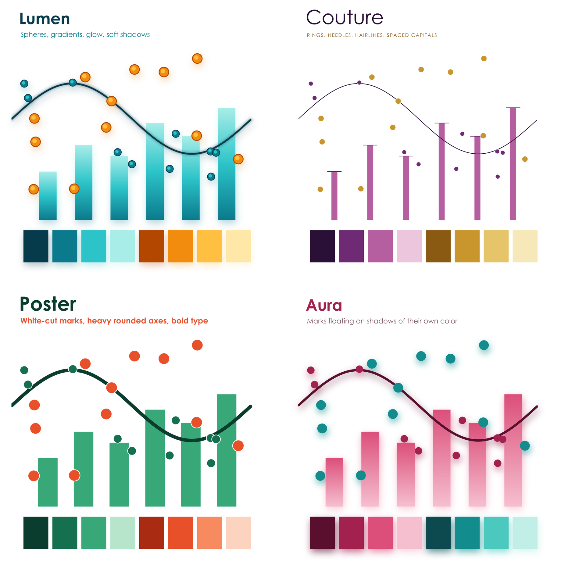
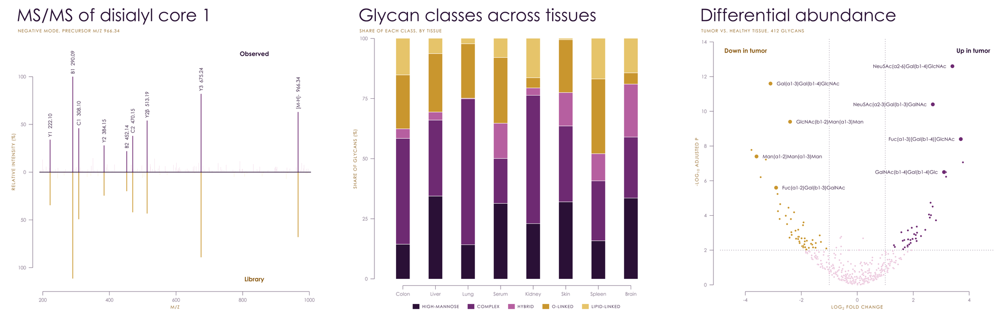
Gradients run through the marks, points are glossy spheres, lines glow, and everything rests on soft shadows.
Hairline axes held away from the data, slender needle bars, large light titles, and spaced capitals.
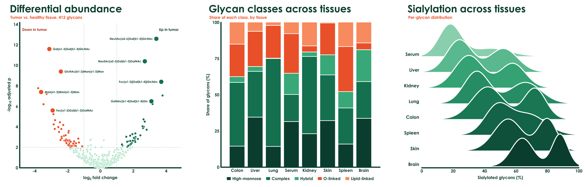
Heavy rounded axes, big bold type, and thick solid marks cut apart by crisp white gaps.
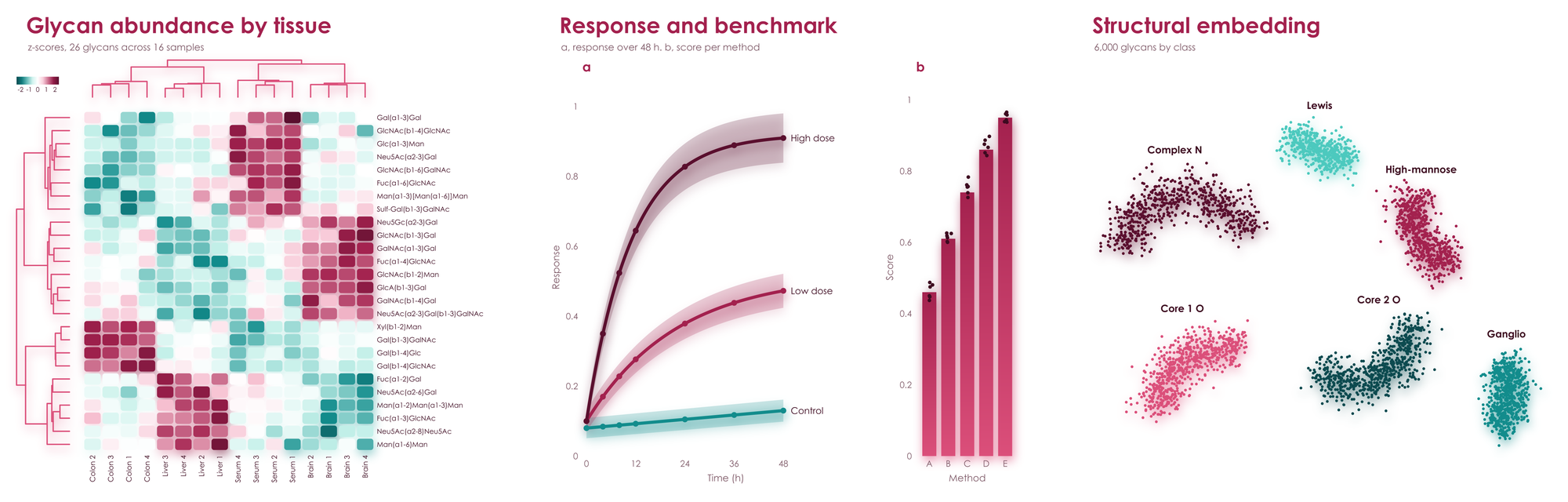
Marks float on soft shadows in their own color, above rounded heatmap cells, with no axis lines at all.
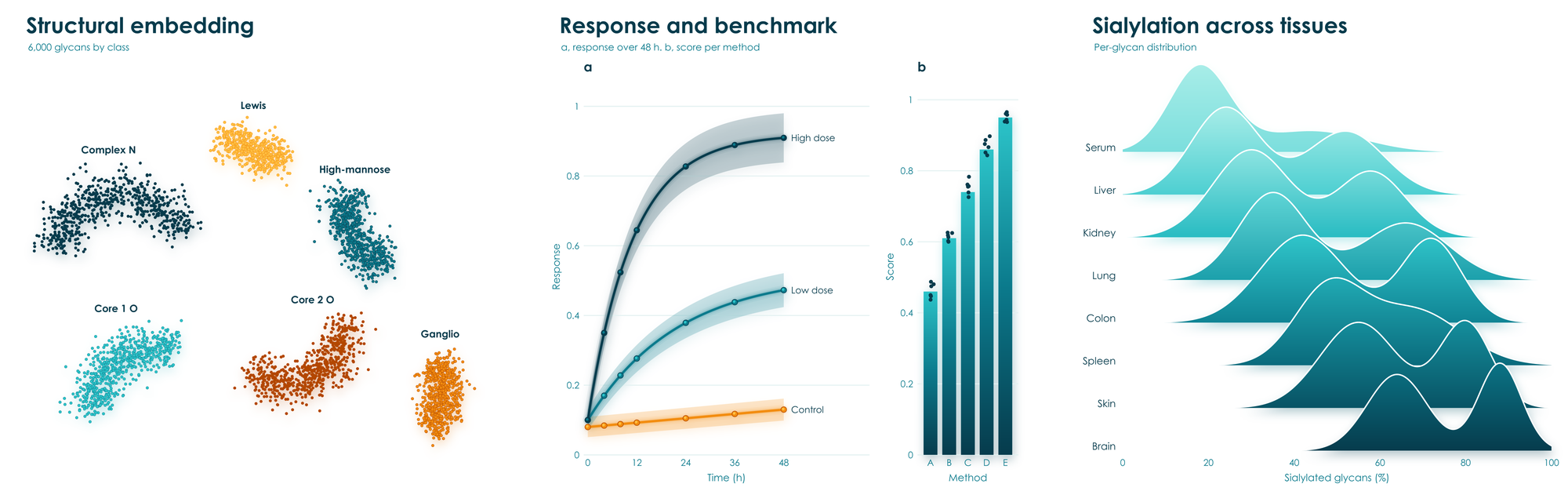
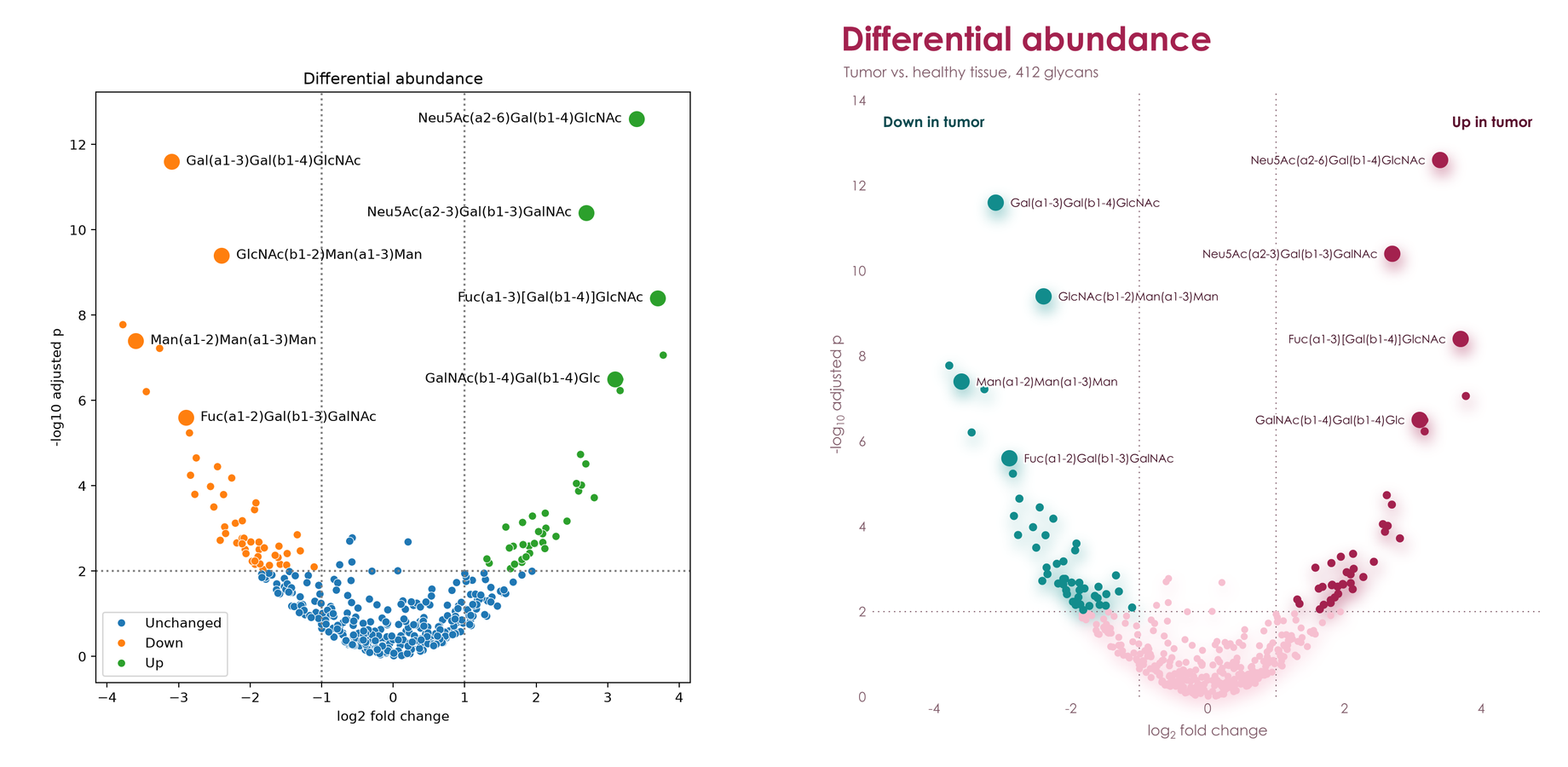
The same data and the same labels, with no styling on either side: matplotlib and seaborn on the left, viscose on the right.
viscose shares its renderer with glycowork's GlycoDraw, so a plot can carry real SNFG drawings as sharp as the rest of the figure, in PNG, PDF, and SVG.
from glycowork.motif.draw import annotate_figure

ax.annotate('Neu5Ac(a2-6)Gal(b1-4)GlcNAc', (x, y), offset = (12, 0), svg_label = True)
fig.save('volcano.svg')
annotate_figure('volcano.svg', filepath = 'volcano.pdf', compact = True)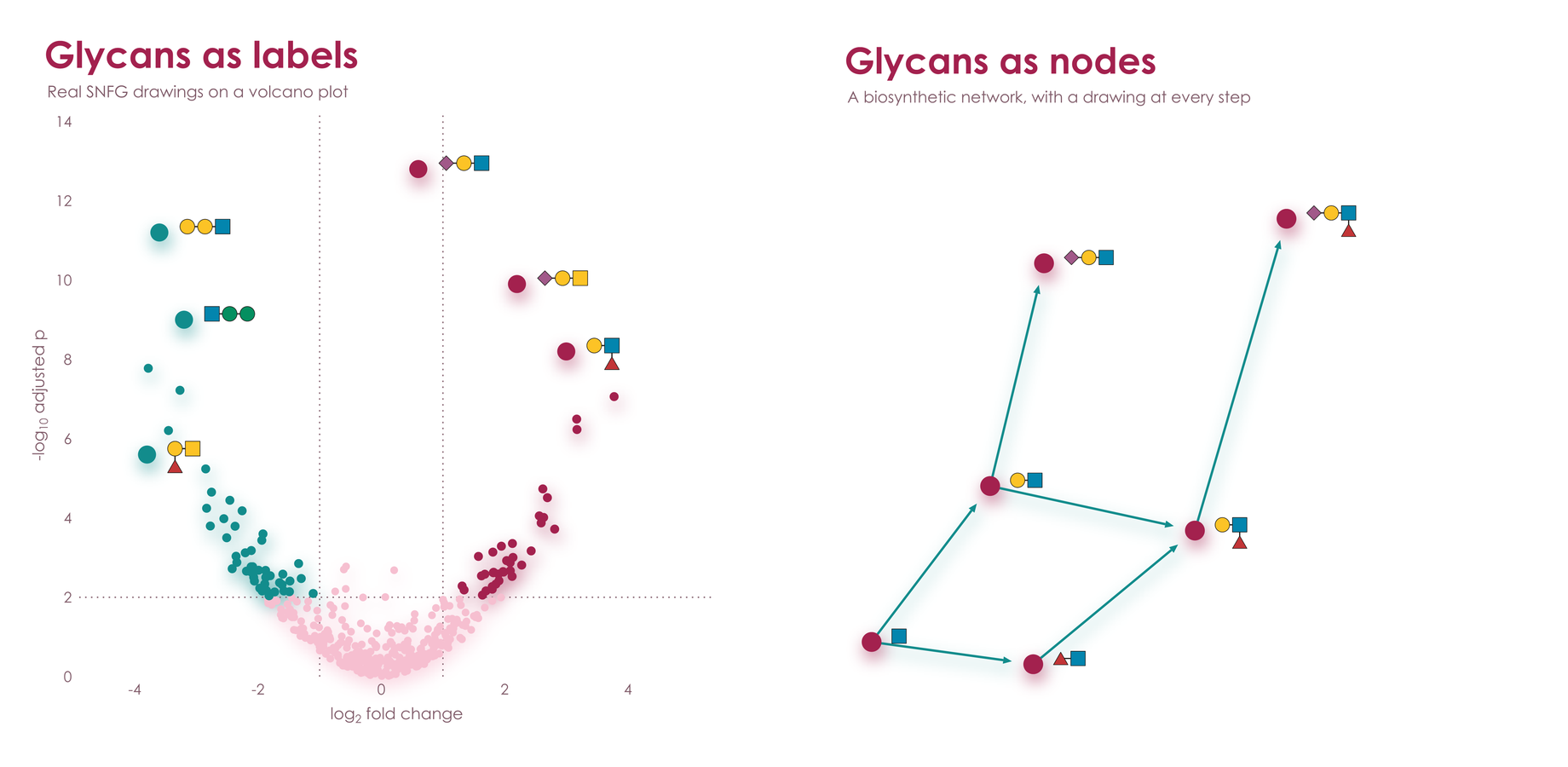
hue, style, and size take one value per point and build the legend for you, as seaborn does.
ax.scatter(x, y, hue = stage, style = source, size = abundance,
           hue_label = 'Stage', style_label = 'Source', size_label = 'Abundance')
ax.text(0.02, 0.98, 'F = 4.2\np = 0.003', axes_fraction = True, va = 'top')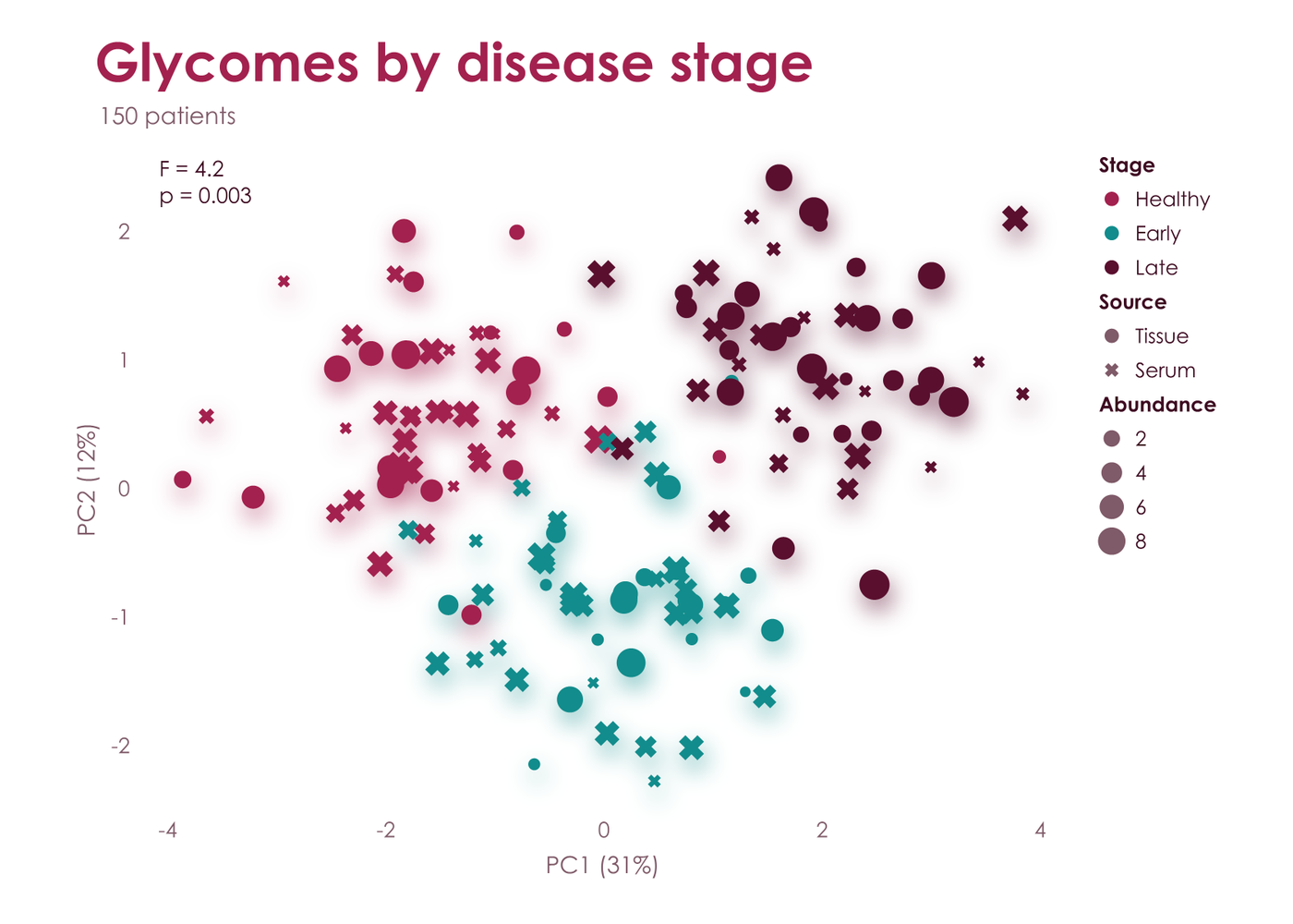
Clustermaps come with both dendrograms and a color bar. Hand over a DataFrame and it brings its own labels.
fig, heat = vc.clustermap(df, palette = 'aura', title = 'Glycan abundance by tissue', colorbar_label = 'z-score')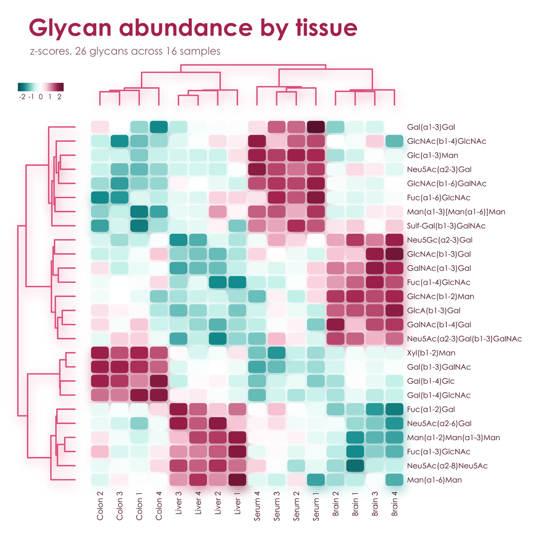
| Plots | plot, scatter, bar, barh, stacked_bar, hist, fill_between, errorbar, stem, hlines, arrow, heatmap, ridgeline, dendrogram, axhline, axvline, and vc.clustermap |
| Markers | o, s, D, ^, v, X, P, and *, all with the palette's effects |
| Annotation | text, annotate, legend, and colorbar, with _{sub} and ^{super} in any text |
| Layout | Colliding tick labels turn and thin themselves, labels move to the side with room, legends wrap, and the page grows for anything that needs it |
| Output | fig.save writes PNG, PDF, or SVG from the same geometry, with marks, gradients, and text as real vectors in PDF and SVG |
| Display | fig.show() works inline in Jupyter and slate, and in the system's image viewer from a terminal, with CI and coding agents kept silent |
| SVG hooks | gid on arrow and scatter names elements for hover text and scripting |
| State | None hidden: a figure is an object, with no current figure and nothing to close |
No compiled plotting stack, no backends, and no font cache. For vector output, viscose is often many times faster than matplotlib and seaborn, and its files can be far smaller. At 300 dpi, in Poster:
| matplotlib and seaborn | viscose | |
|---|---|---|
| Dependencies | Nine extra packages, 42.5 MB | numpy and glycorender, with 0.11 MB of its own code |
| Clustermap, 300 x 100, PDF | 1.57 s, 587 kB | 0.02 s, 79 kB |
| Clustermap, 300 x 100, SVG | 1.40 s, 5,943 kB | 0.02 s, 182 kB |
| Clustermap, 26 x 16, PDF | 0.11 s, 22 kB | 0.01 s, 26 kB |
| Three lines with a legend, PDF | 0.03 s, 12 kB | under 0.01 s, 13 kB |
| Scatter, 100,000 points, PDF | 0.96 s, 1,524 kB | 0.19 s, 644 kB |
| Scatter, 412 points, PNG | 0.18 s, 147 kB | 0.20 s, 180 kB |
matplotlib's compiled rasterizer is still about twice as fast on most PNGs, and the soft shadows of Lumen and Aura add about half a second. To rerun the full comparison, wins and losses alike, use benchmarks/compare_matplotlib.py.
vc.set_palette('aura') changes the default for every figure. A library that builds on viscose calls vc.default_palette('aura')
instead, which gives way to the choice of whoever uses it. In any palette, refer to its shades as a0 to a3 and b0 to b3, dark
to pale, or as ink, muted, and faint; hex and CSS color names work too. fig.pal.groups(3, 2) gives categories grouped by hue,
here three shades of one and two of the other, and fig.pal.contrast(n) alternates between the hues for categories that have to stand
apart, as scatter(hue = ...) does.
A palette of your own is two hues, three text colors, and whichever effects you like:
vc.register_palette(vc.Palette('midnight', ['#14213D', '#27477E', '#5C85C5', '#C4D5EE'], ['#8F5B00', '#D08C00', '#F2B83B', '#FBE5B0'],
                               '#14213D', '#5A6478', '#E6EAF1', point = 'sphere', bar = 'deep', shadow = 0.4))
fig, ax = vc.subplots(palette = 'midnight')
Century Gothic is used where it is installed, and glycorender's bundled Comfortaa elsewhere.
examples/gallery.py draws seven standard figures in every palette, examples/features.py draws one sheet of features per palette, and examples/readme_figures.py draws every image on this page.